1 variants of PSO
1.1 PSO-1
In PSO-1, we just keep the local part in the SPSO. When the next position of each particle is sampled from the global search range, we continue sampling until the next position of each particle is in the local range. So, the sampling range is as following.
![]() 0
0
![]()
where
![]()
![]() 0
0
![]()
where
![]()
![]()
where
![]()
1.2 PSO-2
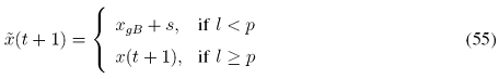
In PSO-2, we randomly generate a particle close to the current best particle in every generation and each dimension with a threshold p which is drawn in the interval [0,1]. Meanwhile we keep the velocities of the particles calculated by SPSO and use them in the next generation. s is randomly drawn from an uniform distribution over the interval [-r,r], and r is the radius of the area around the global best position xgB in the whole population. r is determined according to the attributes of the test functions. When l<p, the actual position ![]() (t+1) would be calculated. Otherwise, x(t+1) will be as the same as that in SPSO. This operation is conducted in each dimension for all particles.
(t+1) would be calculated. Otherwise, x(t+1) will be as the same as that in SPSO. This operation is conducted in each dimension for all particles.
The essence of PSO-2 is to shorten the difference between the current position of a particle and the the global best position in the whole population with a certain probability. Then, the range of sampling can be shortened to a smaller range [-r,r] around the global best position with the probability p, by which, the ratio of the global and local search capability can be tuned by r and p.
1.3 PSO-3
The essence of PSO-3 is adjusting the particles to search the solution space more pertinently. We increase the probability of particles landing into the range around xgB , keep the probability of particles flying far from xgB, and decrease the probability of particles wandering around the small range containing xgB. In such a way, we give the particles who wandered near around the range of xgB a clearer job, which is joining in the range to enhance the local search. In other words, we give all the particles only two choices, either landing very near xgB to enhance the local search ability or landing far from xgB to keep the global search capability. Such, PSO-3 simply makes the
particles search the space more pertinently and efficiently.
In PSO-3, the velocity is used to affect the behaviors of the PSO. In every generation, we set a range [-r,r] around the best individual in each dimension. If the particles in the swarm would pass through the range in the next generation, we use a magnifier operator to enlarge the range without changing velocity of particles. Thus, the particles would get a better chance to land into the range, which is able to check the area around the current best individual more precisely. On the other hand, we keep the velocity of the particles so that they are able to fly out of the range in certain generations to maintain the global search ability of SPSO. The transition process of a particle x from the t th to t+1 th generation in each dimension can be schematically expressed as four situations as the following respectively, and in each situation, the position after using the magnifier operator in PSO-3 will be calculated:

r is the radius of the interval with L and R be the left and right boundary, and s is the scale which decides the multiple we want to enlarge the range. s should not be too small, because we must make sure that the particles will not fall into the range too easily and hard to fly out, which lead to a prematurity. On the other hand, r should reduce along with the growth of generations, because we want the best individual to converge inside the range. So, we should fix an initial value for r, from which r reduces linearly to zero. The iterative equation of r is expressed by
![]()
where k is the current iteration number and M is the maximum iteration number we set.
1.4 PSO-4
In PSO-4, two sub-swarms are used for the evolution. One sub-swarm use the standard formula. The other sub-swarm with n particles using the following formula

where r is used to tune the sampling range of X and Y. The two sub-swarms use different sampling range to evolve. So the performance of the PSO should be changed.
2 Experiments
2.1 Experimental Set-up
To test and verify the performance of the proposed variants, fifteen benchmark functions and their corresponding parameters listed in Table I are used for our following simulations. Besides the global optimum of Shaffer f6 function is 1, the global optimum of the other fourteen benchmark test functions are 0. Since in real-life applications the optimization cost is usually dominated by evaluations of the objective function, the expected number of fitness evaluations was retained as the main algorithm performance criterion. The stop criterion, i.e. a maximum number of fitness evaluations is set to
The column 'Ini. Space' in the table shows the spaces where the initializations lie in. For the concrete expressions of the fifteen test functions used in our experiments and more complex and compound benchmark test functions, interested readers visit our lab with site http://www.cil.pku.edu.cn/resources/benchmark_pso/ for details.
2.2 Determination of Parameters for the Proposed Algorithms
The best tradeoff between exploration and exploitation, strongly depends on the functions being optimized: number of local optima and distance to the global one, position of the global optimum in the search domain(near center, near border), size of the search domain, required accuracy in the location of the optimum, etc. It is probably impossible to find a unique set of algorithm parameters
that work well in all cases. So, we will use an tentative method to determine the parameters picking three representative test functions which are sensitive to the parameters from Table I, i.e., the Sphere function with only one optimum or the Rosenbrock function with slow slope, the Schwefel function being rotated, the Ackley function with multi-local optima, and so on.
2.2.1 Determination of Parameters of PSO-2
Two parameters need to be determined: p and r, which denote the probability to generate a particle around the best position and the radius of the interval mentioned above, respectively. We choose three functions to test their effects. Sphere function and Rosenbrock function both have one single optimum, but the former one has a large scale curvature and the later one has a flat bottom. Rotated Rastringrin function has multiple optima all over the searching space.
With p fixed as 0.05, the performance of the PSO-2 on the three functions with different initial value of r are illustrated in Fig1.(a)-(c). It can be seen that when r=0.000001 we get better performance on all those three functions. In Fig1.(d)-(f, with r fixed as 0.000001, we can also conclude that p=0.1 would be a better choice. So, we determine the parameter set be p=0.1 and r=0.000001.
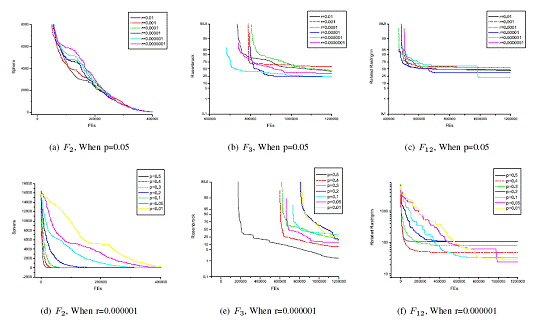
Fig.1 Convergent Performance of the PSO-2 on Sphere, Rosenbrock and Rotated Rastringrin Functions With Different Probability And Radius of the Interval Denoted As p and r, respectively.
2.2.2 Determination of Parameters of PSO-3
Two parameters need to be determined: s and r, which demote the scale of the magnifier operator and the radius of the range in each dimension, respectively. The performances of the PSO-3 on three functions with different scales of the magnifier operator are illustrated in Fig.2. As can be seen, s should not be too small, because we must make sure that the particles will not fall into the range too easily and hard to fly out, which lead to a prematurity, and s=0.5 will be a suitable decision. On the other hand, r should reduce along with the growth of generations, because we want the best individual to converge inside the range. So, we should fix an initial value for r, from which r reduces linearly to zero. The performances of the PSO-3 on four functions with different initial value of r are illustrated in Fig.3. It can be seen that the initial value of r should be 0.3. So in the following experiments, we let s be 0.5 and let r reduce from 0.3 to 0 linearly along with the iteration number.
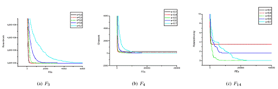
Fig.3 Convergent Performances of the PSO-3 on Four Functions with Different Scales of the Magnifier Operator From 0.3 to 0.7 where r=0.3.
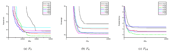
Fig.4 Convergent Performances of the PSO-3 on Four Functions with Different Interval from r to 0 where s=0.5.
2.2.3 Determination of Parameters of PSO-4
Two parameters need to be determined: n and r, which demote the number of particles and the radius of the new sampling range, respectively. The performances of the PSO-4 on three functions with different scales of the magnifier operator are illustrated in Fig.5. As can be seen, s should not be too small, because we must make sure that the particles will not fall into the range too easily and hard to fly out, which lead to a prematurity, and s=0.5 will be a suitable decision. On the other hand, r should reduce along with the growth of generations, because we want the best individual to converge inside the range. So, we should fix an initial value for r from which r reduces linearly to zero. With r fixed as 0.3, the performance of the PSO-4 on the three functions with different number of particles are illustrated in Fig.5(a)-(c). It can be seen that when n=5 we get better performance on all those three functions. In Fig.5(d)-(f), with n fixed as 5, we can also conclude that r=0.3 would be a better choice. So, we determine the parameter set be n=5 and r=0.3.
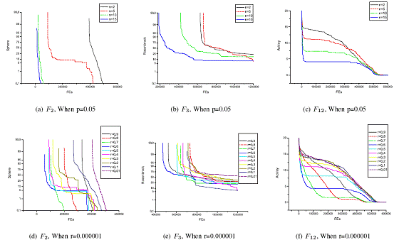
Fig.5 Convergent Performance of the PSO-4 on Sphere, Rosenbrock, and Ackley Functions With Different Number of Particles and the Radius of the New Sampling Range, Denoted As n and r Respectively.
2.3 Performance Comparisons Among Four Variants and SPSO on Benchmark Test Function s
The performance comparisons among the proposed PSO-1 to PSO-4 and SPSO are shown in Fig.6. The convergent curves on fifteen typical benchmark test functions shown in Fig.~\ref{begin} are drawn from the averaged values of independent 50 runs. In such a way, these curves can give the stable performance of the PSO-1 to PSO-4 and SPSO completely and reliably. As we can see from these figures that the proposed PSO-1 to PSO-4 has much faster convergence speed and more accurate solution than that of the SPSO on all fifteen benchmark test functions.
Furthermore, in order to verify the validation and efficiency of our PSO-1 to PSO-4, in Table II, we give the statistical means and standard deviations of our obtained solutions of the fifteen benchmark test functions listed in Table I, by using the proposed PSO-1 to PSO-4, and the original SPSO, over 50 independent runs, respectively. As can be seen, the proposed PSO-1 to PSO-4 has more accurate solution than that of the SPSO on all fifteen benchmark test functions.
Specifically, the relationship of the convergent speed among the the proposed PSO-1 to PSO-4 and SPSO can be observed from Fig.6 as follow
PSO-3 ![]() PSO-4
PSO-4 ![]() PSO-1
PSO-1![]() PSO-2
PSO-2 ![]() SPSO
SPSO
where ![]() denotes the faster speed of convergence. While the relationship of the global exploration capability among the the proposed PSO-1 to PSO-4 and SPSO can be observed from Table II as follow
denotes the faster speed of convergence. While the relationship of the global exploration capability among the the proposed PSO-1 to PSO-4 and SPSO can be observed from Table II as follow
PSO-2![]() PSO-1
PSO-1 ![]() PSO-3 =PSO-4
PSO-3 =PSO-4 ![]() SPSO
SPSO
where ![]() denotes the stronger global exploration capability. = denotes the equal global exploration capability on the test functions. Because it can be seen from Table II that the PSO-1 achieves better global solution than SPSO on ten test functions. PSO-3 achieves better global solution than SPSO on nine test functions. PSO-4 achieves better global solution than SPSO on nine test functions. While the PSO-2 achieves better global solution than SPSO on all of the fifteen test functions. Therefore, it can be concluded that the proposed four variants, i.e., PSO-1 to PSO-4, speed up the convergence tremendously, while keeping a good search capability of global solution with much more accuracy. All of the simulation results in our experiments show that the four variants based on the analyses of the PSO give a promising performance.
denotes the stronger global exploration capability. = denotes the equal global exploration capability on the test functions. Because it can be seen from Table II that the PSO-1 achieves better global solution than SPSO on ten test functions. PSO-3 achieves better global solution than SPSO on nine test functions. PSO-4 achieves better global solution than SPSO on nine test functions. While the PSO-2 achieves better global solution than SPSO on all of the fifteen test functions. Therefore, it can be concluded that the proposed four variants, i.e., PSO-1 to PSO-4, speed up the convergence tremendously, while keeping a good search capability of global solution with much more accuracy. All of the simulation results in our experiments show that the four variants based on the analyses of the PSO give a promising performance.
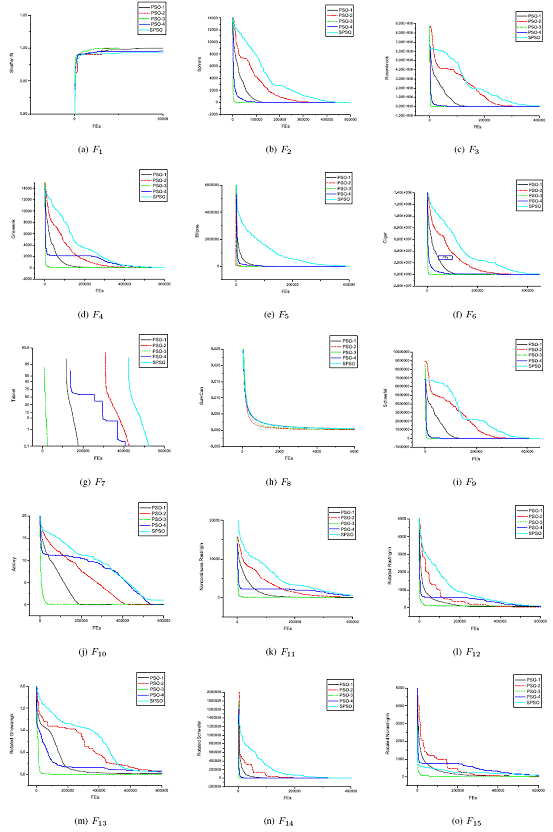
Fig.6 The Averaged Performance of the PSO-1 to PSO-4 and SPSO on F1-F
